Flow-Based Market-Coupling functionality

Introduction

The ongoing market development in the European power system including the Nordic system, requires a further development of decision support tools for stakeholders in the power markets. One of the significant developments in the Nordic system is the implementation of Flow-Based Market-Coupling (FBMC).

The introduction of FBMC is a significant methodological change in the provision of exchange capacity to the market. Instead of Net-Transfer-Capacities (NTC) per transmission corridor, TSOs provide FB constraints in the form of Critical-Network-Elements (CNE), consisting of available capacity (RAM) and a set of Power-Transfer-Distribution-Factors (PTDF) to the market. Example data and data from external parallel runs is published at JAO (https://publicationtool.jao.eu/nordic) and among others applied for assessment of the FB functionality.

Method

The main difference, when going from an NTC based market clearing to a flow-based market clearing is the description of the transmission system. While an NTC based market clearing uses a transport model with transmission corridors, the flow-based market clearing applies a PTDF description. For a more detailed explanation see also [1].

Both NTC constraints and FB constraints define a value for the maximum flow. However, for NTC the flow is just on a corridor and depends on the export/import of two connected areas, while the flow for FB depends on the net position of all areas within the synchronous system. Within NTC maximum transmission constraints are only defined for corridors between areas, while in FB maximum flow constraints are defined for Power Transfer Corridors (PTC) or Critical Network Elements (CNE), that can be between areas or lie within an area. Both flow constraints are addressed as CNE in the following. The resulting optimisation problems for NTC and FBMC have the following forms:

Objective function: Maximise social welfare

Subject to:

\[ ∑ (\text{Net Position}) = 0, \]

\[ \text{NTC or FB constraints.} \]

where the NTC and FB constraints are defined below.

Definition of NTC and FB constraints

The NTC and FB constraints only refer to one direction of transmission/flow. This means that a maximum limit (no minimum limit) is defined. The NTC restrictions are:

\[ F_f \le F_f^{max}, \forall \text{$f$ in $F$} \tag{1} \]

where \(F_f\) is the transmission for corridor \(f\) and \(F\) is the set of all transmission corridors. The power balance in each area is the balance between supply \(P_g\) and demand \(D_l\) in the area as well as export and import \(F_f\):

\[ ∑_\text{$g$ in $G_a$} P_g -∑_\text{$l$ in $L_a$} D_l - ∑_\text{$f$ in $From_a$} F_f + ∑_\text{$f$ in $To_a$} F_f = 0,\forall \text{$a$ in $A$}, \tag{2} \]

where \(a\) is an area and \(A\) is the set of all areas. Based on the power balance the net position for each area can be defined based on supply and demand as:

\[ NP_a = ∑_\text{$g$ in $G_a$} P_g -∑_\text{$l$ in $L_a$} D_l ,\forall \text{$a$ in $A$}, \tag{3} \]

or based on export and import as:

\[ NP_a=∑_\text{$f$ in $From_a$} F_f - ∑_\text{$f$ in $To_a$} F_f = 0,\forall \text{$a$ in $A$}, \tag{4} \]

FB constraints are:

\[ ∑_\text{$a$ in $A$} PTDF_{a,c}*NP_a ≤RAM_c ,\forall \text{$c$ in $CNE$}, \tag{5} \]

where PTDFa,c is the zone-slack PTDF and RAM is the Remaining Available Capacity defined for each CNE.

Inserting the Net position \(NP_a\) equation (4) into the FB constraints equation (5) yields:

\[ ∑_\text{$a$ in $A$}PTDF{a,c}*\left(∑_\text{$g$ in $G_a$} P_g -∑_\text{$l$ in $L_a$} D_l \right)≤ RAM_c ,\forall \text{$c$ in $CNE$}. \tag{6} \]

However, if export and import variables are defined in the market description, the constraint can be written as:

\[ ∑_\text{$a$ in $A$} PTDF_{a,c}*\left(∑_\text{$f$ in $From_a$} F_f - ∑_\text{$f$ in $To_a$} F_f\right) ≤RAM_c ,\forall \text{$c$ in $CNE$}. \tag{7} \]

The advantage of the latter formulation is that there normally is a lower number of export/import variables defined in the market problem than supply and demand variables, especially with a detailed description of numerous power plants. Thus, the constraints as formulated in (7) are implemented in the EMPS.

Input data necessary for FB restrictions in EMPS

The definition of FBMC in EMPS requires input data. While a conventional EMPS dataset can span over several synchronous power systems, including AC and DC connections, the FBMC functionality is only defined for one synchronous area. Hence, the set of areas within the synchronous system and the set of AC lines between the subset of area need to be defined.

• a in A – subset of all areas in the synchronous system (AC system)

• f in Toa and f in Froma – AC transmission corridors within the synchronous areas (HVDC lines are not included in this subset)

The reason for not including HVDC lines in the subset of transmission corridors is that these HVDC lines are part of the dispatchable load and generation, when calculating the net position for the defined areas. Figure 1 depicts a schematic for the calculation of the net position considering AC and HVDC lines.

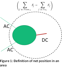
The transmission on the HVDC lines is dispatchable independently from the flow in the AC system. However, maximum, and minimum transmission limits need to be defined on the HVDC lines in MASKENETT.DATA. See example with HVDC lines in separate areas here :doc:FBMC example <fbmc_example>.

In addition to the set of areas and lines, the set of CNEs needs to be defined. These CNEs can come from different sources, such as generated from a detailed grid model or data published at JAO. The definition of a CNE at least needs the RAM and PTDF factors for each area in the AC system.

Implementation

The new functionality of FB constraints is implemented in the EMPS version 10 and requires a user license.

EMPS consists of two main parts:

• The strategy phase, in which water values are calculated on an aggregate area level given historic inflow scenarios.

• The simulation phase, in which the system is simulated for all the historic weather scenarios including the detailed hydropower dispatch based on the drawdown heuristics.

The implementation of FBMC in EMPS is done in the simulation phase. This means the additional FB constraints are added in the market problem with aggregated hydropower, which is solved for the total system. Due to the type of constraints, the problem becomes a general LP and can no longer be solved with a network solver.

Figure 2 shows the schematic of the solving procedure for the simulation phase in EMPS. This is an iteration between the aggregate area optimisation and the reservoir drawdown heuristics. The new FB functionality is marked red in the figure.

Figure 2: The schematic of the solving procedure for the simulation phase in EMPS with the new FBMC constraints in red.

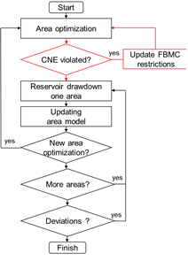
As there already is an iterative approach for solving the area optimisation, new FB constraints are added iteratively. First the area optimisation is solved without any FB constraints. After the area problem is solved, violation of FB constraints is checked. Violated constraints are added and the area problem is re-solved. This approach limits the number of FB constraints added to the problem, the LP size and keeps solution time short.

FBMC in EMPS

The additional FBMC functionality is implemented in the simulation part of EMPS. This means the additional functionality is available in samtap (and related variants samtap_cplex, samtap_cplex_ms_mpi etc). Since the LP changes its structure, a general LP solver needs to be applied. This requires the utilisation of COIN-OR CLP or CPLEX. It is recommended to use CPLEX, if available, to reduce solution time.

FBMC input

Using the FBMC functionality requires additional input. This input is in a dedicated input file, called ptdf_constraints.h5. A snapshot of the file is shown in the Figure 3.

Figure 3: The schematic of the solving procedure for the simulation phase in EMPS with the new FBMC constraints in red.

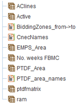
The description of each group is shown in Table 1.

\(Lines\) is the number of lines in MASKENETT.DATA. \(nEMPS\_Areas\) is the number of areas in the EMPS dataset. \(nPTDF\_Areas\) is the number of bidding zones in the AC-grid. \(Week_s\) and \(Week_e\) are the start and end week of the simulation.

Table 1: Example of EMPS dataset areas and the PTDF price areas.

Input Group	Description	Dimensions	Values
Active	CNEC is active or not active	4: [\(CNEs\), \(Scens\), \(Weeks\), \(LP\)]	Integer: \(x \epsilon [0, 1]\)
AClines	List of maskenett lines between PTDF Areas in the synchronous system/AC system	1	Integer. \(x \epsilon Lines\)
EMPS_Area	List of area numbers of the EMPS dataset in the synchronous system mapped to PTDF_Area	1	Integer. \(x \epsilon nEMPS\_Areas\)
PTDF_Area	List of area numbers with defined PTDFs in the synchronous system mapped to EMPS_Area	1	Integer. \(x \epsilon nPTDF\_Areas\)
No. weeks FBMC	Number of weeks in the simulation with FBMC constraints. Switching to NTC constraints for the remaining weeks.	1	Integer. \(x \epsilon [Week_s, Week_e]\)
ptdfmatrix	Zone to slack PTDFs – Values describe flow increase on the CNE in response to a 1 MW increase of the net-position of the bidding zone.	5: [\(CNEs\), \(nPTDF\_Areas\), \(Scens\), \(Weeks\), \(LP\)]	Float. \(x \epsilon [-1.0, 1.0]\)
ram	Remaining available margin (available transmission capacity for trade)	4: [\(CNEs\), \(Scens\), \(Weeks\), \(LP\)]	Float. \(x > 0.0\) [MW]

where \(CNEs=\)Number of CNEs, \(nPTDF\_Areas=\) number of areas in AC-grid, \(Scens=\) Scenarios, \(Weeks=\) Weeks, \(LP=\) Intra-week time-steps or Load Periods of the simulation.

When defining FB constraints based on CNEs, the NTC variable constraints based on MASKENETT.DATA are relaxed for all lines in the AC-grid and the flow is only restricted by the FB constraints. Therefore, note that the exchange results (economic flow) on SAMRES.h5 are not necessarily meaningful. Use the physical flow (flow_values) on FBMC.h5.

Mapping the EMPS areas and PTDF areas

The areas in the EMPS dataset and the price areas do not necessarily match. For example, a dataset can have 11 EMPS areas in Norway while the JAO data has 5 price areas in Norway as shown in Table 2.

Table 2: Example of EMPS dataset areas and the PTDF price areas.

EMPS Area Numbers	EMPS Area Names	PTDF Area Number	PTDF Area Name
1	Ostland	1	NO1
2	Sorost	2	NO2
3	Hallingdal	3	NO3
4	Telemark	4	NO4
5	Sorland	5	NO5
6	Vestsyd
7	Vestmidt
8	Norgmidt
9	Helgeland
10	Troms
11	Finnmark

Therefore, we need a mapping between them. Table 3 shows an example mapping of the areas for a Sintef dataset. Here we have put the EMPS areas into the PTDF areas based on the geographical location.

Table 3: Example of EMPS dataset areas and the PTDF price areas.

EMPS Area Numbers	EMPS Area Names	PTDF Area Number	PTDF Area Name
1	Ostland	1	NO1
2,4,5,6	Sorost, Telemark, Sorland, Vestsyd	2	NO2
8	Norgemidt	3	NO3
9,10,11	Helgeland, Troms, Finnmark	4	NO4
3,7	Hallingdal, Vestmidt	5	NO5

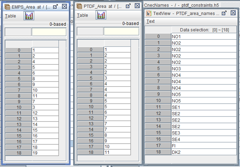
Using this mapping the EMPS_Area and PTDF_Area on the FBMC input file becomes as shown in Figure 4.

Figure 4: Mapping the EMPS_Area and the PTDF_Area. The PTDF_area_names are shown on the right.

Mapping of the ACLines from MASKENETT.DATA

The AClines group in the input file is a list of connections between the PTDF price areas mapped to the lines in MASKENETT.DATA. As an example AClines from a SINTEF dataset is shown in Figure 5.

Figure 5: connections between the PTDF price areas mapped to the lines in MASKENETT.DATA.

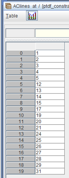
where the mapping of interconnections (only the first 13 lines are shown) in MASKENETT.DATA and AClines is shown in Table 4.

Table 4: Example of EMPS dataset areas and the PTDF price areas.

Line Number	From	To	EMPS Area	PTDF Area	AClines
1	‘OSTLAND’	‘SOROST’	NO1	NO2	1
2	‘OSTLAND’	‘HALLINGDAL’	NO1	NO5	2
3	‘OSTLAND’	‘TELEMARK’	NO1	NO2	3
4	‘OSTLAND’	‘NORGEMIDT’	NO1	NO3	4
5	‘OSTLAND’	‘SVER-MIDT’	NO1	SE3	5
6	‘SOROST’	‘TELEMARK’	NO2	NO2
7	‘SOROST’	‘SORLAND’	NO2	NO2
8	‘HALLINGDAL’	‘VESTMIDT’	NO5	NO5
9	‘TELEMARK’	‘SORLAND’	NO2	NO2
10	‘TELEMARK’	‘VESTSYD’	NO2	NO2
11	‘SORLAND’	‘VESTSYD’	NO2	NO2
12	‘VESTSYD’	‘VESTMIDT’	NO2	NO5	12
13	‘VESTMIDT’	‘NORGEMIDT’	NO5	NO3	13

Scenario dependent FBMC constraints

Scenario dependent FBMC constraints is activated if the number of scenarios \(Scen\) on the input file is equal to the number of scenario in the simulation. The following groups must have equal number of scenarios on the input file:

• Active,

• ram,

• ptdfmatrix.

Switching from FBMC constraints to NTC constraints in simulation

It is possible to run simulations with FBMC constraints for a user specified number of weeks before switching to NTC constraints for the remaining simulation period. This can be activated by specifying a number higher than 0 for group “No. weeks FBMC” in the input file. For example, the simulation period in a dataset is set to 156 weeks and “No. weeks FBMC” is set to 52 weeks. The simulation will then use FBMC constraints for the 52 first weeks and switch to NTC constrains from week 53 to 156.

Treatment of the HVDC-lines

HVDC lines must be handled separately from the AC-grid (see background in - Input data necessary for FB restrictions in EMPS). We recommend the creation of separate HVDC line areas at each connection point. These areas need their own PTDFs and virtual PTDFs (see for example the JAO publication tool).

Running the simulation with FBMC

As with the conventional EMPS, the simulation is done with samtap. The samtap variants available are linked with the LP-solvers coin or CPLEX and with or without parallel processing. To run samtap with FBMC functionality, it must be started with the extra parameter FBMC. The following commands need to be run depending on the samtap version available Table 5. The FBMC functionality can also be activated in the LTM application.

Table 5: samtap variants.

Serial Processing	Parallel Processing
samtap FBMC	samtap_ms_mpi FBMC
samtap_cplex FBMC	samtap_cplex_ms_mpi FBMC

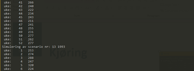
Furthermore, there are no extra parameters / inputs necessary in the interface of samtap. Figure 6 shows the output to command prompt from samtap with FBMC functionality. The output shows the week being simulated and the number of additional FB constraints that are included in the LP for each week.

Figure 6: Output to screen from simulation with FBMC functionality.

Numerical differences for the samtap variants

The FBMC results are stored with high precision format (“double-precision floating-point format” or 64 bits float). However, the communication routines for parallel processing in EMPS use lower precision format (“single-precision floating-point format” or 32 bits float). Therefore, numerical differences on the results will occur. For the highest precision use serial processing variants and for faster simulation use parallel processing. Increasing the precision for parallel processing is possible but will require extra funding. Increasing the precision will also increase the memory usage.

In addition, the two solvers can give solution differences.

Results for FBMC

The FBMC functionality output data is stored in two files:

File Name	Description
FBMCStats.dat	Overview of CNEs that are binding and their dual values
FBMC.h5	dual_values – detailed dual value for each CNE
	flow_values – detailed flow for each CNE

Detailed description of the output is given in the following sections.

FBMCStats.dat

This file contains an overview of the binding CNEs and their dual values as shown in Figure 7. The first line in the file contains the number of simulated scenarios. The following lines show the binding CNEs (flow on CNEs at maximum capacity). Each line contains three columns:

1. CNE number, according to the list of CNEs in ptdf_constraints.h5 (first dimension)

2. Average (over all scenarios) annual sum of the dual value for the CNE

3. Total number of times the CNE is binding over all scenarios

Figure 7: Output to screen from simulation with FBMC functionality.

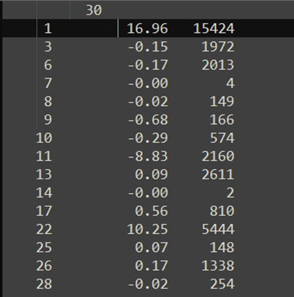
An application of the results in FBMCStats.dat is to identifying bottlenecks of the AC-grid, both frequency and cost.

FBMC.h5

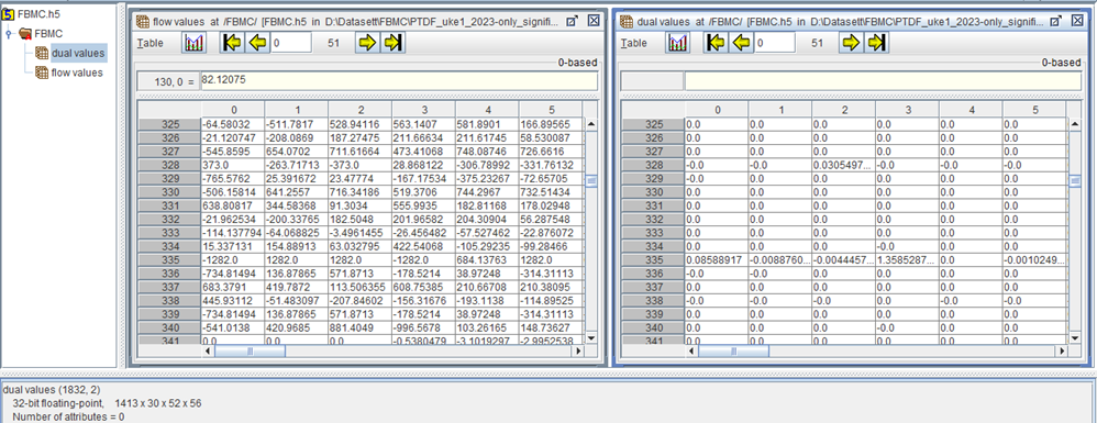
This results file contains detailed information of the dual values of the FB constraints and flow values on the CNEs for all time steps of the simulation. Both the results dual_values and flow_values have 4 dimensions: Number of CNES, Scenarios, Weeks and Load periods per week. Figure 8. shows a snapshot of the file from HDFView.

Figure 8: Output to screen from simulation with FBMC functionality.

Penalty variables in FB constraints

Penalty variables are added to the FB constraints to secure a valid solution of the LP-problems. These variables have a very high penalty cost. If these variables are used the prices from the solution is probably very high. We recommend re-running the simulation after adjusting the RAM for the CNE where the penalty variable is active. However, in our testing of FBMC the penalty variables have not been activated.

If they are activated a log-file is written to the dataset folder called “fbmc-log.dat” with information on the CNE, timestep and flow on penalty variable.

Calculation time

The calculation time will increase using the FBMC functionality. The inclusion of FB constraints requires a switch to the generation of general LP-problems which are more computationally demanding than the network problems solved with NTC constraints.

For example, using the Sintef dataset with 1400 (!) CNEs defined in the input file and FBMC constraints active for all weeks, the computation times are:

• NTC constraints: 10 minutes

• FB constraints: 1 hour and 17 minutes

using the CPLEX solver.

Bibliography

[1] Statnett, Svenska Kraftnätt, Fingrid and Energinet.dk, “Methodology and concepts for the Nordic Flow-Based Market Coupling Approach,” 2019.