Production discharge curve

Fig 1. schematically illustrates an overview of a hydropower module where the tailrace elevation is below the highest regulated reservoir level (HR) in the downstream reservoir. The figure has the heads [m]:

• Maximum head (Hmax): The difference between the HR and the tailrace elevation of the module downstream.

• Minimum head (Hmin): The difference between the lowest regulated reservoir level (LR) of the module and the HR of the module downstream.

• Gross head (Hnom): The nominal gross head is defined by the user, and is often referred to the average reservoir level. The discharge curve referes to this head.

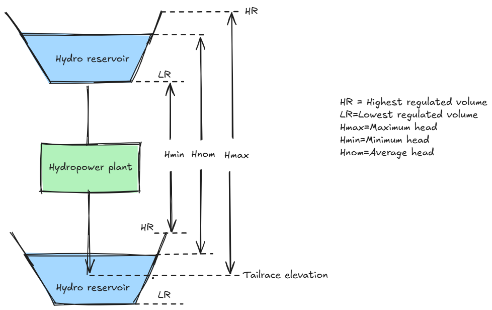
Fig. 1: Visualisation of the head between two modules

Warning

Wrong reference for the gross head for the discharge curve may cause poor results.

Fig. 2 schematically illustrates a description of a reservoir volume curve (reservoir volume as a function of elevation above sea level) and a plant production-discharge curve (pq-curve). In the model, the pq curve is modelled as a piecewise linear curve that shows the relationship between production and the associated discharge.

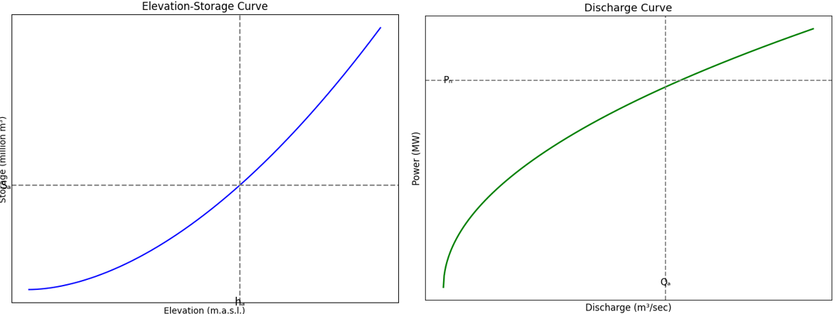
Fig. 2: Reservoir volume and production-discharge curve

If the reservoir level is known, it is possible to find the elevation and thereby the actual head (Ha) from the reservoir volume curve. At a discharge (Qa) the production Pnom(Qa), referred to the gross head, is found from the discharge curve.

Production referred to the arbitrary head and discharge is calculated in LTM using the equation:

(1)\[Pa = \frac{Ha}{Hnom} Pnom(Qa)\]

where

Pa = Production at arbitrary head and discharge [MW]
Ha = Actual head [m] (from reservoir volume curve)
Hnom = Nominal gross head [m] (often refered to the average reservoir level)
Pnom(Qa) = Production at discharge referred to nominal gross head [MW]

Warning

1. Lack of comprehension of the relationship between the gross head, tailrace, the reservoir volume curve and the discharge curve has caused major problems for new users.

2. LtmApi: the attributes reservoir volume_curve, gross_head and tailrace_elevation are required! See Plant.

(CLI LTM-core: allows for omitting the registration of the reservoir volume curve, nominal gross head and tailrace elevation when the head does not affect the result. But not the LtmApi.)

Piecewise linear functions

Piecewise linear functions are used to describe time dependent constraints and functional connections. Time dependent constraints:

• Reservoir constraints: Maximum/minimum allowable reservoir level for specific periods specified in percentage of the maximum reservoir.

• Reservoir reference curve: curve for guiding the reservoir volume with time in buffer reservoirs and energy inflow calculation (bound simulation)

• Discharge constraints: Maximum/minimum allowable discharge (m3/s) for plant discharge.

• Minimum discharge (m3/s) for bypassed water.

NB. The specified constraint for a week is always referred to the end of the week.

Functional connections:

• Production (p) - discharge (q) curve: Production [MW] as a function of discharge [m3/s]

• Discharge constraints: Rated discharge [m3/s] as a function of head [m]

• Volume curve: Reservoir volume [Mm3] as function of elevation [masl]

Time dependent constraints

This section describes how to register data to piecewise linear functions describing time dependent constraints:

• Reservoir constraints: Maximum/minimum allowable reservoir level for specific periods specified in percentage of the maximum reservoir.

• Discharge constraints: Maximum/minimum allowable discharge (m3/s) for plant discharge. Minimum discharge (m3/s) for bypassed water.

See the TxyLin for usage in the LtmApi.

In the example a data period of 156 weeks is assumed. We will distinguish between cyclic and non-cyclic repetition of the piecewise linear functions. Fig. 3 illustrates an example of a curve that is cyclically repeated, while Fig. 4 illustrates a curve that is not cyclically repeated.

LTM calculates discharge/reservoir volume for an arbitrary week using linear interpolation at the segment of the curve for that week.

Note that the specified constraint for a week is always referred to the end of the week.

Cyclic repetition

It is not necessary to specify piecewise linear functions for the whole data period to model time dependent constraints. If the constraint does not change from year to year within the data period is it sufficient to only describe the function for the first year of the data period. The curve/constraint will then be cyclically repeated for all years of the data period.

Table 1 shows an examples of data for the discharge which is illustrated in Fig. 3 as line 1.

Table 1: Weekly discharge table

Week number	Discharge (m³/s)	Discharge (m³/s)
1	15.0
17	15.0	15.0
18	10.0	10.0
39	10.0	10.0
40	15.0	15.0
52	15.0

In Table 2 the maximum reservoir level should be equal to 0 % at the end of week 17, less or equal to 70 % at the end of week 30 and less or equal to 85 % at the end of week 39 for a maximum reservoir constraint. Illustrated in Fig. 3 as line 2.

Table 2: Weekly maximum reservoir level

Week number	Maximum reservoir level (%)
17	0.0
30	70.0
39	85.0

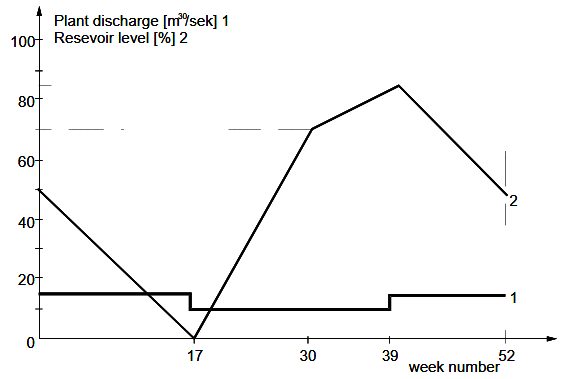
Fig. 3: Cyclic piecewise linear curve, i.e. repeated each year for the whole data period

Non-cyclic time dependent constraints

Fig. 4 illustrates a piecewise linear curve that is not cyclically repeated. In this case draining of the reservoir is planned because of maintenance work in the period from week 127 to week 142, performed by using the maximum reservoir constraint. Data for the curve illustrated in Fig. 4 are shown in Table 3.

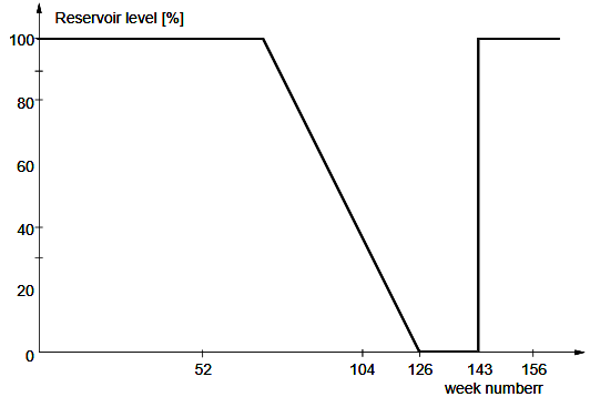
Fig. 4: Non-cyclic piecewise linear curve for maximum reservoir constraint

Table 3: Weekly maximum reservoir level not cyclically repeated.

Week number	Maximum reservoir level (%)
1	100.0
69	100.0
126	0.0
142	0.0
143	100.0
156	100.0

Maximum discharge

Fig. 5 illustrates a piecewise linear constraint that describes the relationship between the head [m] and the maximum discharge (m3/s). Before the discharge constraint can be registered the tailrace elevation, nominal head and volume curve must be defined for the module. If the tailrace elevation is below the HR in a downstream reservoir, the data must also be registered for the downstream module for the maximum discharge to be described correctly. This configuration is described in Fig. 1, where we find:

• Maximum head (Hmax) The difference between the HR and the tailrace elevation [m] of the module.

• Minimum head (Hmin) The difference between the LR and the HR of the module below [m].

The maximum discharge must be registered correctly between the heads Hmax and Hmin (maximum 10 breakpoints). LTM requires the lowest breakpoint of the discharge curve is referred to a head of 0 metres with an associated discharge of 0 m3/s.

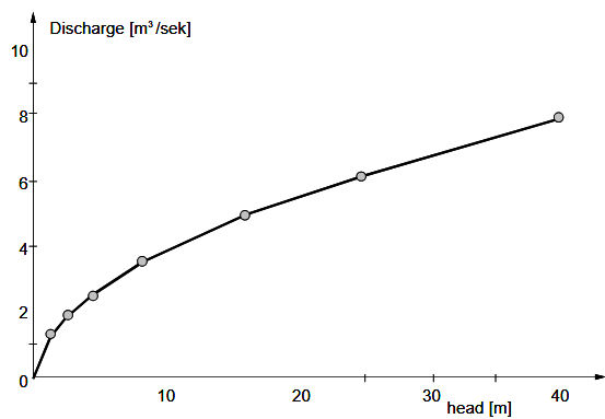
Fig. 5: Piecewise linear curve describing rated discharge as a function of the head