Time in the LTM-core

This section covers the many concepts of time in the LTM-core the LtmApi. Many of these concepts feel natural, but some of the concepts are known to introduce confusion among the users, therefore we recommend dedicating time to understand these concepts.

Introduction

The Long-Term Models (LTM) build and solve weekly optimisation problems in sequence for a defined period, the period is normally from 1 to several years (modelling maximum is 25 years). The models take into account uncertainty in weather and prices in defined scenarios. The weather data is normally based on historical times series.

Due to the week centered modelling philosophy of the LTM models, each year in the LTM-models are not defined by the earths time in orbit around the sun. But each year contains 52 weeks, 364 days or 8736 hours and is refered to as an EFI year and each week as an EFI week. The EFI year start in week 1 and ends after week 52. The EFI week’s first day is Monday and the last day is Sunday, it contains 168 hours and a user defined number of time steps which is described here: LTM-core short-term periods.

LTM-core long-term periods

Below is the important long-term periods in the LTM-core:

1. Simulation period

2. Historical period

3. Data period

4. Water value period

we recommend making an effort to understand and remember the concepts. Below is an illustration of the period “hierarchy” and how they relate to each other.

where:

Data period >= Water value period >= Simulation period.

Ideally, these periods should overlap, but the reality is that this is not always possible depending on the start and end of the periods and the system modelling.

Simulation modes

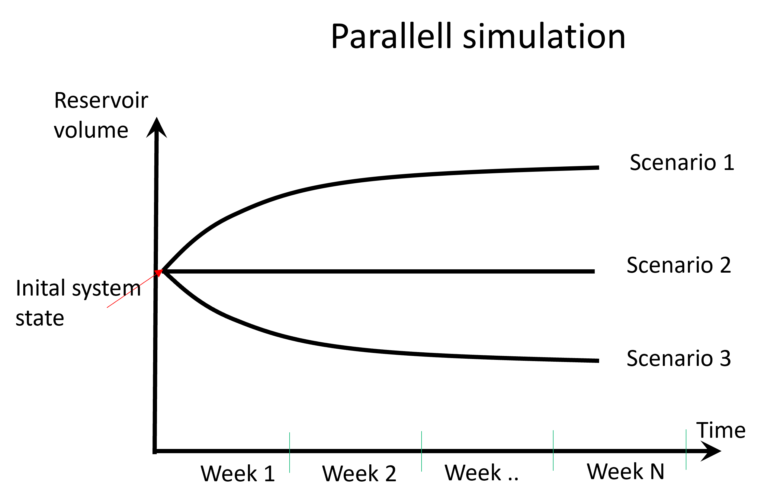
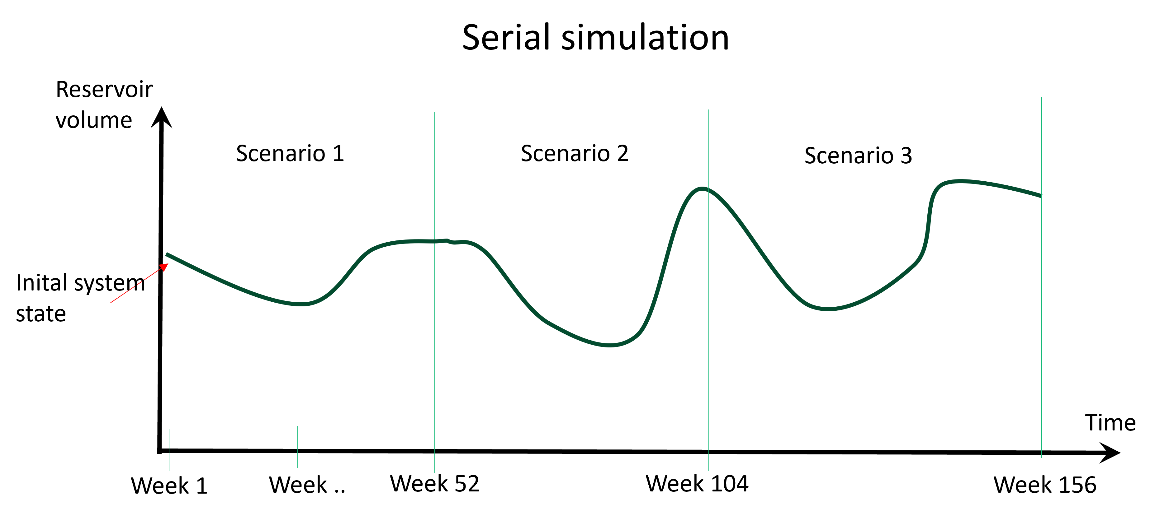
Further there are two simulation modes available, for illustration of the modes a simple example is provided where the uncertainty is represented by three scenarios:

1. Parallell simulation - all scenarios starts from the same system state given as input boundary conditions. All scenarios start at the same time and are simulated for a specified simulation period (week 1 to week N). This mode is used for day-to-day operation. All scenarios are independent of the others and can be simulated in parallell using parallell processing to increase calculation speed.

2. Serial simulation - the scenarios are simulated in series, only the first week of the first scenario use input boundary conditions to set the system state. The simulation period for each scenario is 52 weeks. Boundary conditions are passed on from the weekly solution as input to the next week to set the system state until all scenarios are solved. Simulation speed up using parallell processing is not possible. This mode is typically used for investment and system analysis.

Simulation period

The simulation period is the period for which the power system is simulated using the LTM-models and power system results can be extracted. The period must be defined within the bounds of both the data period and the water value period.

Historical period

Used to define the period of historical data input to the model, such as:

• inflow

• temperature

• wind

• solar

• exogenous price

Scenarios

The scenarios, representing the modelling uncertainty, are defined based on a combination of the mentioned periods. Where the simulation period defines the scenario start point and scenario length. For serial simulation the scenarios are always 52 weeks (1 EFI year).

Data period

The period where data is needed in order for the LTM-core to run successfully. It represents the outer limits of the timeline of the system modelling. The period must as a minimum start and end at the same time as the simulation period and the water value period, but may span a longer period in both directions. For example the data period can be 3 years, starting in 2024. All timeseries and other data must be complete for the 3 year period from 2024 - 2027.

By default this period is calculated by the LtmApi based on the simulation period.

Important requirements:

• The data period starts at the beginning of an EFI-year (beginning of week 1)

• The data period ends at the end of an EFI-year (end of week 52)

See examples in Data period

Water value period

Period defining the bounds for the strategy calculation (or water value calculations). The period must be shorter or equal to the data period and longer or equal to the simulation period. In some cases, the simulation may require data that extends both before and after the specified simulation period. For example in the strategy calculation it may be necessary to look sufficiently far ahead in the calculation process, requiring data to be available several weeks beyond the simulation period.

LTM-core short-term periods

The LTM-core short-term periods within an EFI week are:

1. Accumulated timesteps

2. Sequential timesteps

which are used to specify the number of timesteps per week. The short-term periods are active for all weeks of the simulation period.

Each timestep can span from 1 to 168 hours and anything in between. It is up to the user to define the timesteps per week and the distribution of hours per timestep. The number of timesteps per week can greatly affect the computation time of the simulation. The higher the time resolution the higher the computation time. If several hours of the week have similar (or equal) demand and supply of power the hours can be collected into one timesteps.

Sequential timesteps

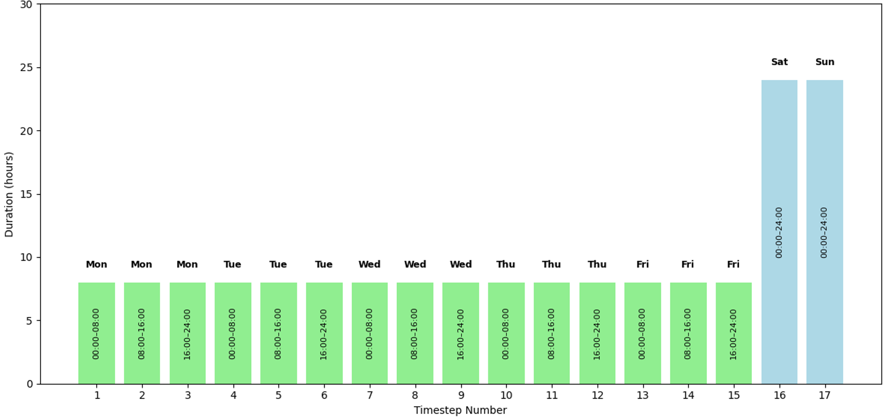
For example one can choose to have 3 timesteps per day, each timestep has 8 hours intervals 0:00 - 8:00, 8:00 - 16:00 and 16:00 - 24:00 from Monday to Friday. Also assuming equal supply and demand all hours of the weekend, we put Saturday and Sunday in one timestep of 48 hours. When using sequential timesteps each timestep starts at the beginning of each day at 00:00. Therefore the timestep containing 48 hours in the weekend becomes 2 timesteps of 24 hours. Resulting in a total of 3 timesteps per day * 5 days + 2 timesteps in the weekend and a total of 17 timesteps per week.

Visualised in the figure with sequential timesteps:

Accumulated timesteps

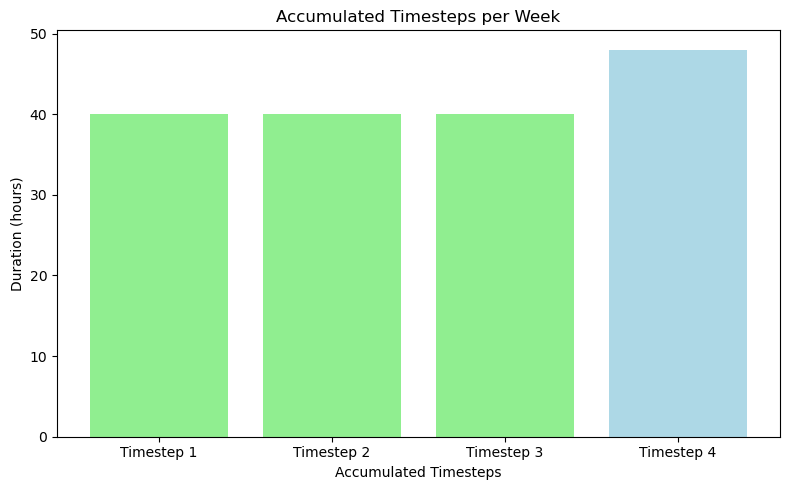
It is also possible to define accumulated timesteps. The reason for using accumulated timesteps is to reduce the total number of timesteps and calculation time. To illustrate the use of accumulated timesteps we continue with 3 timesteps per day in 8 hour timesteps T1 (0:00 - 8:00), T2 (8:00 - 16:00) and T3 (16:00 - 24:00). They are assumed to have equal demand and supply of power for all days from Monday to Friday. The weekend is one timestep of 48 hours.

Illustrated in the figure below (in the same manner as for sequential timesteps):

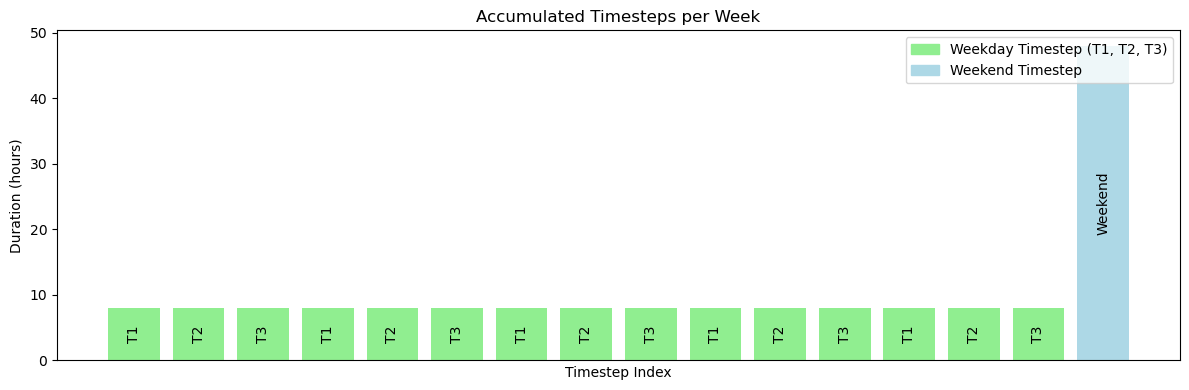
and where we have 5 instances of timesteps T1, T2 and T3 which after accumulation becomes 4 timesteps as shown in the figure below.