Water Value method

This section describes basic philosophy of the water value concept, the calculation assumptions and the water value method. Some approximations are used because of calculation issues or related to the complexity of the complete mathematical formulation are also highlighted. The consequences of these approximations are evaluated where possible.

Philosophy

The objective is to plan operation such that the expected value of the total operation dependent costs subject to imposed constraints are minimized. The total operation dependent costs are:

The operation dependent cost of thermal power generation plus the operation dependent cost of purchasing supplementary power minus the income of occasional power plus curtailment costs,

where occasional power usually means net sales on the spot market. Here a minimization of objective function for the water value method is applied, but it can be reformulated as a profit maximization problem.

This is the philosophical foundation of the term water value.

Illustrative example follows below: Here certain obligations (firm power that must be delivered) are assumed, meaning contractual supply obligations that must be met.

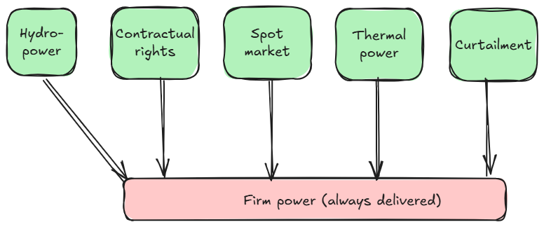
To minimize operation-dependent costs, the guiding principle is to supply the last kilowatt-hour (kWh) from the lowest priced available resource. This requires that all resources be properly priced. Pricing contractual rights, contract repurchase, and thermal units is straightforward. However, curtailment costs must be set higher than the most expensive sales option to prevent purchasing curtailment power only to resell it in the market. The core decision challenge lies in managing reservoirs while considering contractual obligations and the spot market.

By understanding the value of your own water resources, you can determine the optimal strategy for participating in the spot power market, based on prevailing electricity prices. This principle forms the foundation for submitting bids on the spot power exchange. In practice, submitting a bid reflects the producer’s assessment of the value of their reservoir water unless the bid is driven by forced generation.

The value of own water is a function of future development depending on load, market for power and inflow. The value of water is thus no deterministic quantity. It is necessary to introduce a quantity characterizing this uncertainty, and the expected value is the most common one to use. This value is called the water value, and is an expression for the expected marginal value of the stored energy.

Decisions based on water values aim to minimize the expected operational costs, assuming accurate modeling of future market and inflow conditions. However, water value alone does not reveal the consequences of using it as a decision basis. Therefore, simulations using water values as a decision basis is performed to reveal the consequences.

Discussion of assumptions

It is necessary to obtain a realitic model of the power system, for current and future expected developments, when calculating the water values. The future itself is uncertain and it is therefore reasonable to include this uncertainty in the modelling. In the following we discuss the necessary assumptions needed in a water value estimation and also the associated uncertainty.

Elements affecting the water values:

• System state

• Expected load

• Spot market expectation

• Inflow expectation

System state

This applies primarily to the reservoir volumes and the generation capacity. The current reservoir levels are assumed given and future reservoir levels are the free variable for the water value calculation. The generation capacity, as a function of time, represents an uncertainty because it can be dependent on inflow, discharge distribution, constraints and of planned and forced outages. It is in practice difficult to consider the real uncertainty in generation capacity. However, experience indicates that this uncertainty is not important for the water values. Therefore, generation capacity is described as a time dependent deterministic function.

Expected load

In this context, load means firm power supply obligations. The firm power obligations can be described as a time dependent function for future demand. One way to do this is to specify a prognosis for the annual energy, based on an energy demand analysis, as well as a distribution formula for the time variation within the year. This representation assumes that the distribution formula is independent of the absolute level of the firm power. This assumption seems acceptable. It is also possible to include load variation caused by temperature variation if historical temperature series are available.

However, the uncertainty in the annual energy forecast can have significant impact, particularly if the current system is hard pressed. Looking far into the future, e.g. in development planning, the uncertainty in load forecast is increased accordingly. Investigations carried out by EFI indicate that by taking into account uncertainty in the annual energy forecast (stochastic firm power), one would have significant different results compared with what one obtains with deterministic firm power. This applies particularly to development planning. Operational planning is less affected, since the uncertainty in the load is much smaller.

Spot market expectation

The spot power market represents, in many ways, the most difficult element to model in the water value calculations. The uncertainties are significant, and even worse, they are hard to model. The following factors are assumed to contribute to this uncertainty:

• Reservoir conditions in the surroundings

• Inflow conditions in the surroundings

• Foreign markets

• Bottlenecks in the system, both in the grid and on the production side

• Strategic behavior in the surroundings

The first three points represent elements that can be described to some extent, while the last two points pose major challenges for mathematical and logical modeling. Particularly for strategic behavior which is influenced by human judgment, experience, and personal attitudes something that (fortunately?) still escapes precise algorithmic formulation. To model the uncertainty in the spot power market that can reasonably be described, two methods have been developed:

Representing the external environment as a market with stochastic prices (a so-called price series where prices are linked to the inflow series). Representing the external environment using one or more generation models in interconnected operation (the EMPS model).

These representations share the characteristic of establishing a market for power exchange that can be included in the calculation of water value. In today’s models, it is also possible, to some extent, to model bottleneck constraints in the system when describing the external environment.

Inflow assumptions

The value of water is linked to a large extent to expectations of future inflow to the system. In Norway, future inflow must be considered a stochastic variable since the Norwegian system is almost completely dominated by hydropower. The description of the water supply as a stochastic process is a good starting point. A large number of metering stations covering most of the country contain historical observational timeseries for inflow. This can then be used to estimate the inflow for most locations.

Representation of the mean inflow

The basis for evaluating the system’s normal generation ability is accumulated annual inflow from inflow statistics.

This introduces the first uncertainty, deciding the mean inflow. Using the coefficient of variation: \(CV = \sigma/ \mu\), the estimate of mean inflow based on a random n-years series is \(CV / \sqrt(n)\). If the variation coefficient is 0.2 the mean inflow is \(0.2 / \sqrt{n}\).

A 30-year series thus has a probability of 0.3 of reaching an error of 4 %. Put in perspective, the inflow expectation value’s uncertainty is at least the size of the load expectation value’s uncertainty. However, there is not much one can do with this uncertainty, and we must basically require that the water value estimation’s inflow representation has an expectation value close to the mean value of observed inflow.

Representation of the standard deviation

The same reasoning applies when calculating the standard deviation of annual inflow: the inflow model used for water value estimation should replicate the observed inflow characteristics as closely as possible. However, this requirement is difficult to meet. Inflow data exhibits autocorrelation (inflow inertia), whereas the current water value estimation algorithm treats weekly inflows as stochastically independent variables. Consequently, this requirement cannot be satisfied unless fictitious (non-observed) weekly inflow data is introduced into the water value calculations.

Adopting an estimation approach that uses fictitious weekly inflow would likely face skepticism and require extensive additional computations. It would also raise conceptual challenges. Therefore, the decision has been made to use real observed weekly inflows in water value estimations. However, this means that the inflow representation in the water value estimation does not fully match the statistical properties of the observed inflow series. Despite this limitation, the resulting estimates of statistical parameters generally remain within acceptable error margins. For multi-reservoir problems, inflow representation has not yet been fully evaluated. In such cases, both geographic cross-correlation and autocorrelation in inflow must be considered.

Inflow prediction

When incorporated into water value estimations, inflow forecasts serve two main purposes:

• Provide a more accurate expectation value for future inflow

• Reduce uncertainty (standard deviation) in future inflow

The snowpack offers additional information beyond pure statistical analysis for predicting future inflow. This approach is known as spring flood forecasting. When the snowpack is measured, future inflow consists of two components:

• A known part (melted snowpack)

• An unknown part (future rainfall and possible evaporation)

As winter progresses, a larger share of the spring flood volume will come from the known snowpack, while a smaller share will depend on rainfall during the forecast period. Consequently, the uncertainty in the spring flood forecast declines continuously throughout the snow accumulation season, assuming the snowpack estimate is reasonably accurate.

This reduction in forecast uncertainty (standard deviation) is illustrated in Figure 2.

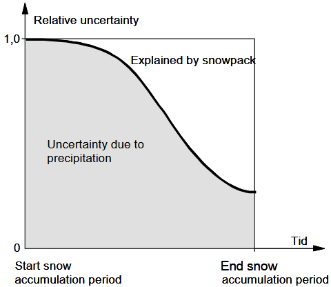
Fig. 2: Example of how the uncertainty in the spring flood forecast is reduced with time.

Spring flood forecasts are volume-based forecasts characterized by statistical parameters such as mean value and standard deviation. To incorporate snowpack information into water value calculations, it must be converted into inflow data. This requires synthesizing inflow series for the spring flood period that reflect the forecast’s statistical properties. These series can then be used to update water value calculations.

Short-term inflow forecasts rely on models that integrate near-term weather predictions. Current weather forecasting capabilities provide realistic horizons of about one week, at least in Northern Europe. Consequently, short-term inflow forecasts have limited relevance for water value calculations. However, they are useful for operational planning, where decisions such as optimal generation for the coming week depend on water values, expected market prices, and anticipated inflow.

The optimization

Water values are derived from an economic optimization problem, where the objective is to minimize the expected operational costs associated with fulfilling given obligations.

The optimization process produces water values, which serve as decision signals for optimal operation. However, water values alone do not provide insight into the consequences of using them as decision signals in operational planning. Therefore, consequence analyses are essential and can be improved by developing simulation models that incorporate market-oriented decisions, such as water values and forecasted inflows.

A key challenge in using operational simulation for consequence analysis is selecting a meaningful simulation sequence. It is important to note that water values are not optimal for a single, randomly chosen inflow sequence. They are optimal for an infinite inflow series with statistical properties similar to those used in estimating the water values. When the same inflow sequence is used in both the simulation and the water value calculation, the water values can be tested against an infinite number of possible events. However, the results of operational simulations carry inherent uncertainty, as each outcome represents a random event drawn from an infinite set of possibilities.

The water value method

It is practical to link the basic description of the water value method to an aggregate model of a hydropower system as shown in Fig 3.

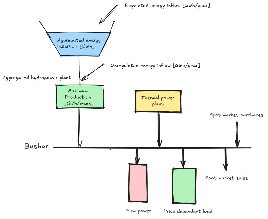
Fig. 3: Vizualisation of the aggregated hydropower model. An aggregated hydropower equivalent model can be made from any detailed hydro power system.

All reservoirs in a detailed hydropower system are aggregated into a single aggregate reservoir, and all plants are combined into one aggregate plant. The firm power supply is specified on a weekly basis, along with the prices and permitted quantities for purchased or sold power and thermal generation. Additionally, the cost of curtailing firm power supply (or repurchasing contracts) is included. Inflow is represented by separate series for regulated and unregulated energy inflow. The transmission grid is modeled as a single busbar. The following section describes the economic optimization process and the estimation of water values.

Mathematical derivation

The objective function form a basis when planning optimal economic operation of a hydropower system. The planning period can be divided into time steps of one week. The weekly optimization problems are solved in sequence from the beginning and to the end of the planning period, providing generation decisions which minimize the total operation dependent costs for the whole planning period.

In Fig 4. and in equation 1 function \(J(x,k)\) represents the expectation value of the total operation dependent costs, from the start of the week \(k\) for a given reservoir energy content \(x\).

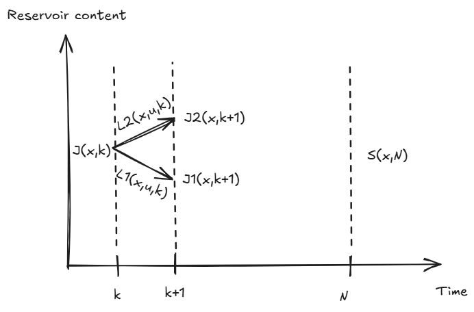
Fig. 4: Vizualisation of the analytical expression for the water value method. Time is on the x-axis and reservoir volume on the y-axis.

(1)\[J(x,k) = S(x,N) + \sum_{i=k}^N L(x,u,i) = L(x,u,k) + J(x,k+1),\]

where \(S(x,N)\) is the cost of the volume change in the reservoir. Meaning the value of the start reservoir volume minus the value of the remaining storage content, as function of the reservoir level \(x\), at the end of the period at time N.

\(L(x,u,i)\) is the operation dependent costs when going from period \(i\) to \(i+1\). \(L(x,u,i)\) includes costs of purchasing power, costs of thermal power generation, costs linked to curtailment of firm power and income from spot power sales.

\(u\) is the energy drawn from the reservoir to produce a certain power \(p\).

The total operation dependent costs at time \(k\) is equal to the sum of all variable costs \(L(x,u,i)\) over the entire period plus the costs of reservoir change \(S(x,N)\). This is also equal to the operation dependent costs the first week \(L(x,u,k)\) plus the total operation dependent costs \(J(x,k+1)\) from time \(k+1\) to the end of the planning period.

Depending on the energy \(u\) drawn from own reservoir, different variable costs \(L1(x,u1,k)\), \(L2(x,u2,k)\), etc. is obtained for a given week. The problem is to find the value of the energy \(u\) drawn resulting in lowest costs.

Optimal management of own reservoirs is achieved when the total operation dependent costs \(J(x.k)\) are minimized with regard to the energy drawn \(u\):

(2)\[min_u J = min_u [L(x,u,k) + J(x,k+1)],\]

found when:

(3)\[\frac{dJ}{du} = \frac{\partial L}{\partial u_k} + \frac{\partial J}{\partial x_{k+1}}\frac{\partial x_{k+1}}{\partial u_k} = \frac{\partial L}{\partial u_k} + \frac{\partial J}{\partial x_{k+1}} (-1) = 0,\]

where the derivative of the reservoir level with regard to the energy release is

(4)\[\frac{\partial x_{k+1}}{\partial u_k} = -1.\]

The condition for optimal strategy for period k is

(5)\[\frac{\partial L}{\partial u_k} = \frac{\partial J}{\partial x_{k+1}}\]

where \(\frac{\partial L}{\partial u_k}\) is the marginal operation dependent costs linked to purchase, sale, curtailment, etc and \(\frac{\partial J}{\partial x_{k+1}}\) is the derivative of the total future operation dependent costs with regard to the reservoir level. This is defined as (marginal) water value at time k+1, \(x_{k+1}\).

With the total operation dependent costs for the entire planning period as a basis, we have shown that optimal management of hydropower within each period (week) can be achieved by trading based on the water value. This means that it is optimal to have the purchase and sales marginal cost equal to the water value.

Therefore, when the water value is known in week \(k+1\) and is to be estimated for a reservoir point in week \(k\), the water value is equal to the water value at the reservoir level in week k+1, assuming optimal operation within the week. This is in accordance with equation (5).

The optimal decision at a reservoir point, m, is in Fig. 5 illustrated for a given inflow during the week in question, assuming the water value is known by the end of the week. This is the inner logic in both the water value calculation and the operation simulation.

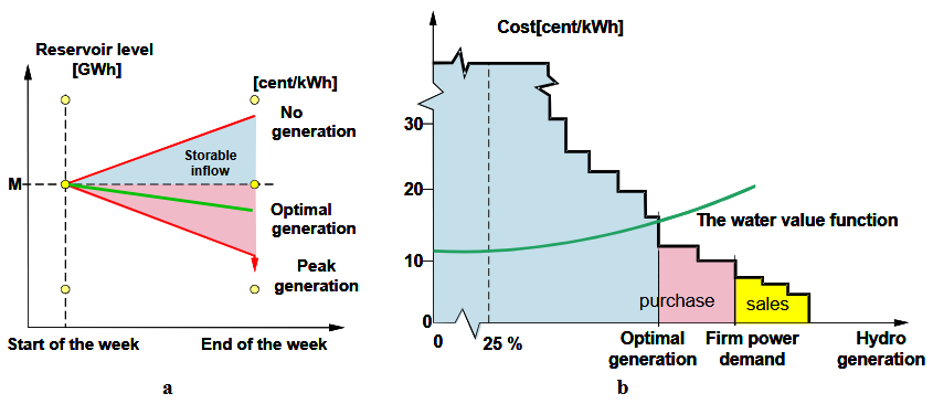
Fig. 5: Example of optimal decision based on the water value.

With a given weekly inflow, the relation between hydropower generation and the weekly resulting water value is calculated. This is shown in Fig. 5a. The calculated function is shown in Fig. 5b.

Marginal operation dependent cost linked to purchase, sales, thermal power generation, curtailment, etc. as a function of hydropower generation (a demand curve for hydropower) is drawn as a stepwise curve in Fig. 5b. To the right of the point for firm power demand the curve represents sale of spot power. To the left of this point the curve represents purchase, thermal power production and rationing.

Optimal hydropower generation is given by the intersection point between the two curves. Knowledge of the inflow has been assumed in this fundamental explanation of the method. This is a simplification of the problem and the inflow’s uncertainty is in practice considered by performing an equivalent calculation for a number of discrete weekly inflows.

Handling the top and bottom in the reservoir

What happens when the reservoir is either full or empty is critical for determining the water value. Near the top of the reservoir, overflow losses occur during periods of high inflow, even under full generation. Water stored at this level has no economic value, so the water value is effectively zero. To avoid overflow, generation can be increased beyond what the end-of-week water value suggests. This means selling power at a marginal price lower than the water value for a full reservoir at week’s end. In such cases, the water value at the start of the week equals the price of the last kilowatt-hour sold, the marginal market price.

Conversely, near the bottom of the reservoir, energy shortages may arise during periods of high demand and low inflow. Here, the water value equals the price of the last kilowatt-hour purchased or curtailed, provided this price exceeds the water value for an empty reservoir at week’s end. Conditions at the reservoir limits strongly influence water value, and these effects propagate inward as calculations progress.

End point values and time horizon

Water value calculation is a form of backward dynamic programming dynamic programming, where the derivative of total costs is stored rather than the total cost itself. Equation (5) assumes that the water value for week k+1 is known. At the end of the planning horizon, however, the water value is unknown and must therefore be estimated or guessed. When the planning horizon is sufficiently long, the current week’s water value becomes independent of the assumed end-point values. In the long run, only the effects at the top and bottom of the reservoir influence water value. This means that the specific end-point guess does not matter, provided the horizon extends far enough into the future.

The reservoir’s degree of regulation determines how far ahead calculations must begin to ensure independence from the initial end-point assumption. For example, if the reservoir inevitably overflows during a peak inflow period, the water value is zero for the entire reservoir at that time. In such cases, it is unnecessary to look beyond the nearest inflow peak. The situation differs for reservoirs with a high degree of regulation.

Instead of guessing the starting value, an iterative process is applied. Assume reliable data for the power system and market conditions can be established for three years ahead. A water value table can then be constructed with 157 columns: the first column represents the water value at the start of week 1 in year one, and column 157 represents the end of week 52 in year three.

Initial values are assigned to column 157, and water values are calculated backward over 52 weeks to column 105. The values in columns 105 and 157 are compared. If the deviation exceeds a specified tolerance, the initial values in column 157 are replaced with those calculated for column 105, and the process repeats. This continues until the desired precision is achieved, after which water values for the remaining 104 columns are computed. The number of iterations depends on both the initial guess and the reservoir’s degree of regulation. For this iterative approach to work, the power system and the relationship between market and energy supply must remain unchanged beyond the start of year three. In other words, water value columns spaced one year apart should be equal. The same result can be achieved by extending identical data far enough into the future so that the outcome becomes independent of the initial guess.

Applying stochastic inflow

The previous description of the water value method assumed that inflow was known. This section briefly explains how the calculation is performed when inflow is stochastic. Assume that the inflow for the given week can be represented by n discrete inflow values, \(t_i\), i=1,…, n with individual probability of occurring, \(p_i\) where

(6)\[\sum_{i}^{n} p_i = 1,\]

The optimal operation within the week is decided for each of these \(n\) inflow values as described before and the water value for each reservoir point, \(k_i\), is recorded. This is indicated in Fig. 6.

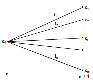
Fig. 6: Illustration of the basis for estimating the water value \(k_0\).

The water value at the desired point is then estimated using the equation:

(7)\[k_0 = \sum_{i}^{n} p_i k_i,\]

To apply this approach, inflow must be treated as an independent stochastic variable. However, it is well known that inflow exhibits serial correlation when short intervals, such as a week, are considered. This is accounted for by assigning different weights to weekly inflow values according to predefined rules.