LTM hydropower modelling¶

The hydropower system is described using standard modules linked via water routes for plant discharge, bypass discharge and overflow/spillway. A module can consist of a reservoir, a plant, inflow, constraints, topology and pump data. Fig. 1 shows an example of a standard hydropower module.

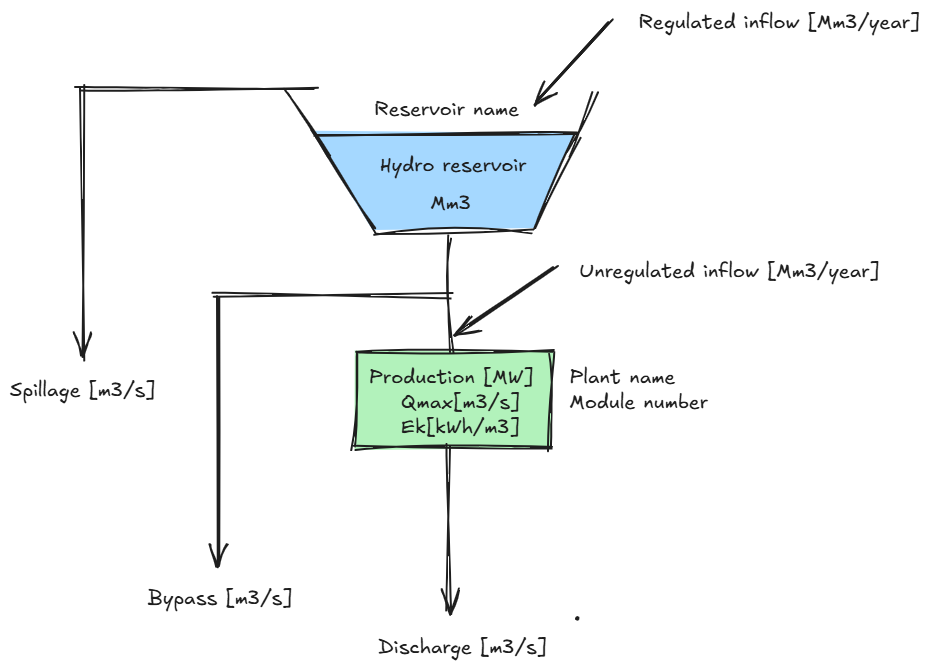
../../../_images/hydro_power_detailed_viz.png — Fig. 1: Standard hydropower module in the LTM.¶

See also the documentation of the LtmApi Hydro power and how the hydropower modules are defined in the LtmApi.

Reservoir¶

The reservoir is described by its volume [Mm3]. In addition it is possible to define the relationship between volume and elevation, the volume curve, as a piecewise linear curve. In some cases it is necessary to define a volume curve (together with tailrace elevation and nominal head):

To adjust the production in relationship to changes in head.

When pumps are connected to a reservoir (to calculate the head).

When the rated discharge is specified to be a function of the head.

Reservoir types¶

The reservoirs can be of either of the two types:

buffer
regulation

Two key piecewise linear curves are used for the reservoirs. The reservoir reference curve [% of maximum reservoir volume] describes the reservoir level as a function of time. The volume curve [m - Mm3] describes the functional relation between reservoir elevation and reservoir volume.

Buffer reservoirs¶

This is operated according to a piecewise linear reference curve for the reservoir level. The reference curve can be specified by the user or automatically calculated by the model. The buffer reservoirs are normally small and poorly regulated with insignificant storage capacity compared to inflow. For the buffer reservoir the storage differs from the reference curve only when this is necessary because of constraints in the system, or when the need for power/energy implies deviation. Small intake ponds to power plants are often defined as buffer reservoirs.

Regulation reservoir¶

Regulation reservoir is managed by a strategy based on rules for the distribution of stored energy in the system. The discharge strategy does not specify anything for the optimal aggregate content of the reservoirs in the system. The optimal aggregate content can be found based on marginal water value of the aggregate reservoir.

In the bounded simulation (regulated and unregulated energy inflow calculation see Energy inflow calculation), both the buffer reservoirs and the regulation reservoirs are controlled by their reference curves. The goal is often set as maximum production for the simulation.

Plant¶

The plant is described using the rated discharge (maximum plant discharge, Qmax in Fig. 1) and the local energy equivalent (Ek in Fig. 1) refered to the average head. For gates the energy equivalent is set equal zero. For plants the relationship between production and discharge is given as a piecewise linear curve (pq-curve), which includes both generator and turbine efficiency and head losses. This curve is referred to a specified head, the nominal gross head. The resulting production for a specified discharge is corrected linearly for changes in head if the reservoir volume curve and the tailrace elevation are defined.

The rated discharge of the gate or plant may be specified as a function of the head. A piecewise linear curve is then defined for the relationship between the rated discharge and the head. Planned outages (for maintenance) are normally modelled by specifying a number of MW as not available for a period. This is converted to a constraint for the discharge capacity of the plant in the model.

Inflow¶

A module can have inflow stored in the reservoir (regulated) and inflow directly to the plant (unregulated). It is assumed in the model that unregulated inflows cannot be stored. If this type of inflow exceeds the discharge capacity, the excess of water is considered to be bypass discharge. If the inflow is storable, it should be defined as regulated inflow.

The inflow is defined by the average annual inflow referred to a specified historical period and connected to a time series that defines the variation from week to week and from year to year.

Inflow unit in the LTM is [Mm3/year]. Note that for the LtmApi the inflow series unit is [m3/s].

Topology¶

The modules in a watercourse are connected by specifying which downstream modules receive plant discharge, bypass discharge and spilled water. The three water routes can go to different modules, or to the ocean. See API Waterways and hydro topology.

Constraints¶

The following constraints that vary with time can be attributed to each module:

Upper limit for the reservoir volume
Lower limit for the reservoir volume
Upper limit for plant discharge
Upper limit for bypass discharge
Imposed minimum discharge through the plant
Imposed minimum bypass discharge

All the constraints can be specified as a piecewise linear variation in time. In addition, it is possible to tie all the constraints for discharge to time series. They will then vary in time with the referred time series.

If the different constraints are in conflict with each other, maximum discharge has the highest priority, followed by the imposed minimum plant discharge and the imposed minimum bypass discharge. Constraints on the reservoir volume have the lowest priority.

The model will try to meet constraints for minimum discharge by first discharging the reservoir directly upstream in the watercourse from where the constraint is defined. If this does not give enough water to meet the constraint, the model will search further upstream in the watercourse until it finds enough water. It is possible to diverge from this strategy if discharge points are specified in a preferred sequence.

Time variable constraints on reservoir volume are interpreted as follows:

When the volume in a reservoir is below the lower reservoir limit, the discharging stops, until the reservoir volume is above the limit. However there is no demand to fill the reservoir with water from a possible upstream reservoir.
When the volume in a reservoir is above the upper reservoir limit, but it is below the physical maximum volume, water is discharged as long as there is enough capacity in the plant or main gate. Bypass will not be used in the local plant, but the discharge can cause loss of water further down in the same watercourse

The rated discharge can be specified as a function of the head (piecewise linear curve).

Pump data¶

Pumping possibilities are described using a linear relationship between the head and maximum capacity for pumping, and the power used for pumping. From where and to where the reservoir water is pumped is defined independently of the defined plant discharge water destination. Two kinds of pumps are possible:

Pumped storage plants: in which the turbines can be reversed to pump water from the plant’s tail water to an upstream reservoir. In EOPS pumped storage plants can be used for seasonal pumping; the model is not designed for daily off peak pumping. In the model a pumped storage plant is defined when the water is pumped back to the same module as the pump is connected to.

Pump stations: the purpose of the pumps is to pump water from one reservoir to another (or to another watercourse) where it is possible to better exploit the water for energy production.

The correct specification of Energy equivalents is important for the pumping behaviour and pumping results.

Usage of Pumps in the LtmApi can be found here Pump object and Pumps in the LtmApi.

Hydraulic couplings¶

The use of hydraulic couplings give greater flexibility in the modelling of watercourses than the standard modules allow for. For example two or more reservoirs can be connected to one plant.

Five kinds of configurations can be modelled:

200 The reservoirs are coupled using an open tunnel or canal. The water is distributed between the reservoirs, only controlled by the pressure head and limits in the transfer tunnel. The configuration is illustrated in Fig. 2.

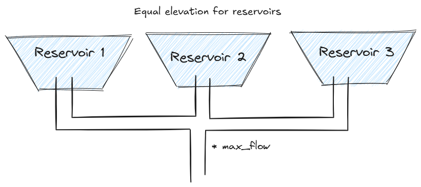
../../../_images/200_v2.excalidraw.png — Fig. 2: Hydraulic coupling type 200 in the LTM. Reservoirs connected using an open tunnel.¶

**300** The reservoirs are coupled using a tunnel or canal with controlled gates. The transfer of water between the reservoirs is controlled by the model’s discharge strategy, limited by transfer capacity. The configuration is illustrated in Fig. 3.

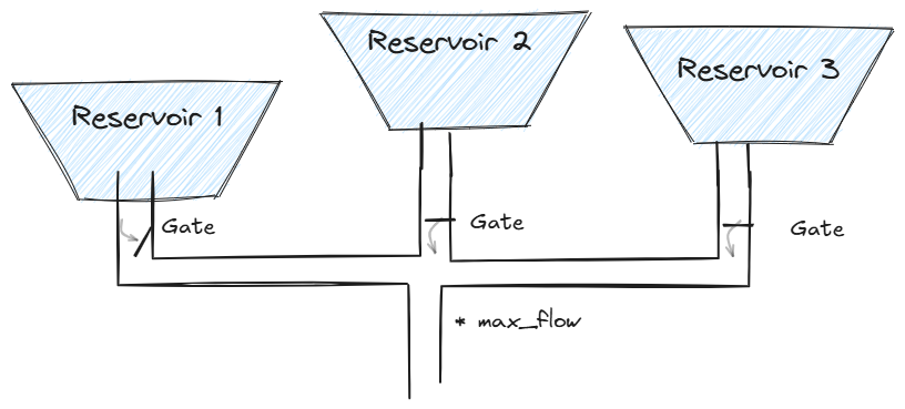
../../../_images/300_v4.excalidraw.png — Fig. 3: Hydraulic coupling type 300 in the LTM. Reservoirs connected using a tunnel controllable by gates.¶

**100** The reservoirs are coupled to a common plant. Direct transfer between the reservoirs is not allowed, but the discharge strategy controls from which reservoir the water is discharged to the plant. This kind of configuration is illustrated in Fig 4.

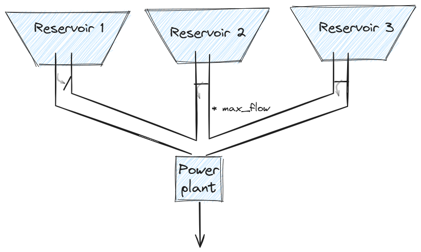
../../../_images/hyd_coupling_LTM_100.png — Fig. 4: Hydraulic coupling type 100 in the LTM. Reservoirs connected using tunnels with gates connected to a common plant.¶

**120** A combination of *200* and *100*, this means reservoirs in parallel that are discharging through a common plant. In addition there is levelling between reservoirs that are controlled by the pressure head outside the plant.

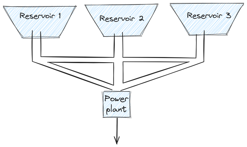
../../../_images/120_v4.excalidraw.png — Fig. 5: Hydraulic coupling type 120 in the LTM. That is parallel reservoirs connected to a common power plant, in addition to flow between the reservoirs. The flow between reservoirs is controlled by the water levels.¶

**130** A combination of *300* and *100*, this means reservoirs in parallel that are discharging through a common plant. The reservoirs are controlled by the discharge strategy. Active control of the transfer capacity by means of gates. Reservoirs which are to be levelled to the same elevation or controlled by the discharge strategy. Visualised in Fig. 6.

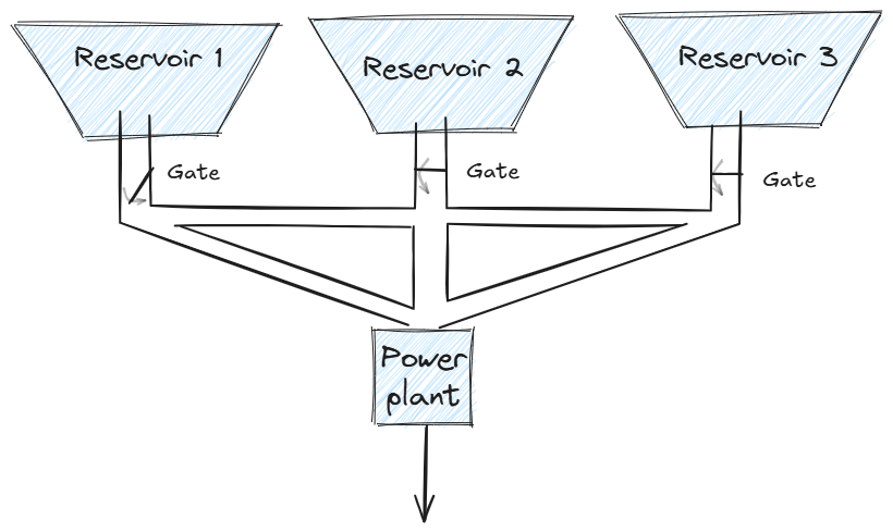
../../../_images/130_v2.excalidraw.png — Fig. 6: Hydraulic coupling type 130 in the LTM. Parallel reservoirs connected to a common power plant, in addition to flow between the reservoirs controlled by hatches.¶

Modelling concept¶

The modelling concept and optimization process consist of two phases. The strategy phase and the simulation phase.

The strategy phase is established using the so-called aggregate hydro model, which is an aggregated model of the detailed hydropower system. See Water Value method and EMPS model strategy and calibration.
The simulation phase of the underlying hydropower system is done using a model of the detailed hydropower system, the detailed drawdown model. See Detailed drawdown

A decision support system should ideally be based on one single integrated optimization process. However, the splitting of the problem in two phases is a necessary simplification to achieve acceptable calculation time.

It is very important that the user has a picture of the model’s composition in order to understand the total concept. The aggregate model will therefore be described as a model of the underlying detailed drawdown model in the following sections.

Detailed model of a water course¶

The modelling of a watercourse is done by attaching standard hydropower modules (shown in Fig 1) using their water routes Water routes for overflow are only drawn when the water does not run to the reservoir immediately downstream. Water routes for bypass are only drawn for modules with bypass discharge constraints. An example water course is shown in Fig. 6. The detailed hydro power model is used in the Detailed drawdown model of the simulation phase.

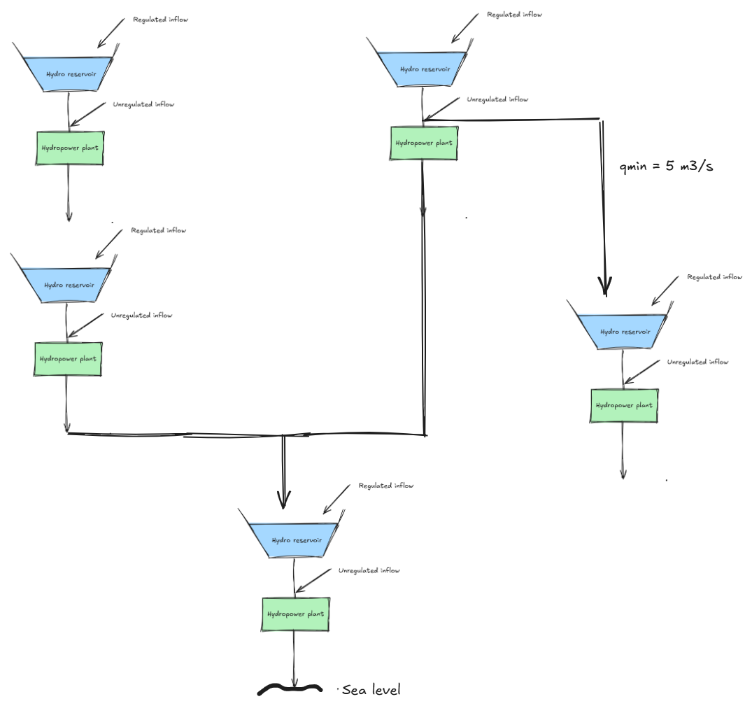
../../../_images/water_course_viz.png — Fig. 6: Example water course coupling the standard hydropower modules to create the water routes.¶

Energy equivalents¶

Two energy equivalents are used in the LTM:

Local energy equivalent
Energy equivalent to sea

In a watercourse with several hydropower modules connected in series it is important to distinquish between the local energy equivalent and the energy equivalent to sea, see illustration in Fig 7.

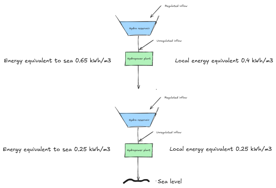
../../../_images/energy_equivalents_viz.excalidraw.png — Fig. 7: Example of the local energy equivalent and the energy equivalent to sea.¶

In the example two hydropower modules are connected in series, each module has a local energy equivalent (on the figure right) and a corresponding energy equivalent to sea (on the figure left). The energy equivalent to sea is the sum of all the downstream local energy equivalents.

Note for energy equivalents:

The local energy equivalent is used when specifying the hydropower modules
The LTM calculates the energy equivalent to sea when appropriate.

Aggregated hydropower model¶

In the strategy phase, the expected value of stored water is calculated as a function of the reservoir and time based on the Water Value method, see also EMPS model strategy and calibration. The water value method is based on stochastic dynamic programming, and requires a simplified model representation of the hydropower. In order to achieve acceptable calculation time, the hydropower system has to be aggregated, so that one gets a single aggregate power station and a single aggregate reservoir. The inflow in the aggregate model is modelled using two energy time series, one for the reservoir and one directly to the plant representing forced generation in the system. Fig. 8 shows the aggregate model for a detailed hydropower system.

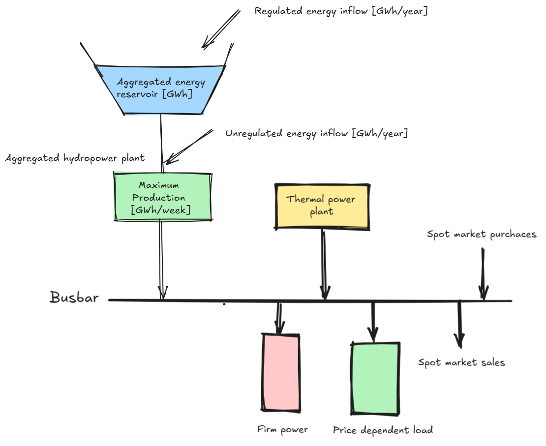
../../../_images/agg_hydropower_viz.png — Fig. 8: Vizualisation of the aggregated hydropower model. An aggregated hydropower equivalent model can be made from any detailed hydro power system.¶

All energy quantities in the aggregate system model have the unit GWh and the energy values are quoted in cent/kWh. This is valid both for values of stored water in the aggregate model and for the market (thermal power, contracts and transmission capacity towards the outside world) connected to the bus bar. The following gives a brief explanation of how the detailed hydropower model aggregates (calculates automatically) to an aggregate model.

The aggregate reservoir¶

The energy from all the reservoirs is summed up to an aggregate reservoir. The energy in a single reservoir is estimated by multiplying the reservoir volume (Mm3) with the sum of the underlying energy equivalent to the sea (kWh/m3). If reservoir constraints are specified for the detail model, these constraints will be transferred to the aggregate model. A minimum reservoir constraint in the detailed model will, as an example, be modelled as a lower reservoir limit. Both upper and lower reservoir limits in the aggregate-model could therefore vary from week to week if reservoir constraints are specified for the detail model. NB. Maximum and minimum reservoir limits in the aggregate reservoir are absolute and can therefore not be violated.

The aggregate plant¶

The maximum generation for each plant is summed to an aggregate plant description. Possible constraints for the individual plant discharge are represented as upper and lower generation limits in the aggregate model, respectively. The aggregate-plant’s maximum generation capacity can therefore vary from week to week, if maximum discharge constraints are specified in the detail model.

Energy inflow calculation¶

Regulated and unregulated energy inflow to the aggregate model is estimated from the detailed drawdown model in EOPS.

Calculation of regulated energy inflow is shown below:

Regulated energy inflow =
                            Sum production (including purchased load factor contracts)
                          - unregulated inflow
                          - energy used for pumping
                          +/- increase/reduction in sum reservoir volume

Calculation of unregulated energy inflow is shown below:

Unregulated energy inflow =
                              Production from unregulated inflow to power plants
                            + production due to minimum discharge and bypass constraints
                            + forced production to avoid overflow
                            - energy used for pumping to avoid overflow