Samnett input file references
The samnett files are:
styredata.nett: Samnett config file
KOMBSNITT.DAT: Monitored interconnections, flow boundaries and outages
nordel_x.dat: Network description, oplast-format
EFI-SNITT.DAT: Power grid electric division of areas
EFI-PROD-1.DAT: Hydropower coupling to grid
EFI-PROD-2.DAT: Hydropower coupling to grid (more than one connection point)
EFI-FAST.DAT: Firm load coupling to grid
EFI-PREF.DAT: Market steps, thermal generation coupling to grid
EFI-MODRED.DAT: HVDC connections
EFI-AREA.DAT: Aggregation of areas
EFI-VIND.DAT: Wind power
linjerevisjon.csv: Line outages
Interconnections between areas in the EMPS is found in the MASKENETT.DATA and must be considered when specifying KOMBSNITT.DAT and EFI-SNITT.DAT.
Samnett - power market simulation and detailed grid analysis
This guide is based on the user guide [1].
Introduction
Samnett combines power market simulation and detailed grid analysis. Although Samnett exists as a separate program, it is tightly integrated with the EMPS model and should ideally be seen as a functionality in the EMPS model. It is therefore assumed that the user has some knowledge of the EMPS model before reading this guide. The documentation of the EMPS and EOPS models should therefore serve as companions to this user guide. A brief description of the EMPS and the integration of Samnett is provided below.
Samnett as Part of the EMPS model
The EMPS model comprises two parts: strategy evaluation and system simulation. The strategy evaluation part computes noncoupled water values for each area with hydropower. These calculations are based on stochastic dynamic programming per area, with an overlaying hierarchical logic applied to treat the multi-reservoir aspect and the interconnection between areas. In the system simulation part, the optimal operational decisions for a sequence of historical weather scenarios are found taking the water values from the strategy evaluation part as input. The system simulation can be performed with or without Detailed Drawdown (Norwegian: “tappefordeling”).
The Samnett program performs a system simulation with Detailed Drawdown and grid analyses. Note that Samnett does not involve the computation of water values since it covers system simulation and not strategy evaluation. The water values computed in the strategy evaluation serve as input to Samnett.
The Samnett code is identical to the EMPS program for system simulation with Detailed Drawdown, but with the addition of integrated grid analysis. The system simulation is illustrated in Figure 1, showing the logic for solving the weekly decision problem for a specific week in a specific inflow year. When solving the weekly decision problem, the EMPS model combines Area Optimization and Detailed Drawdown to reach a solution. The Area Optimization is formulated as a linear programming (LP) problem, where hydropower is aggregated per area. From the solution of the Area Optimization, the aggregated hydropower generation for each area is disaggregated to the detailed hydropower for that area through the Detailed Drawdown. In case the disaggregation results are not satisfactory, the equivalent hydropower representation is updated, and the Area Optimization is run again.
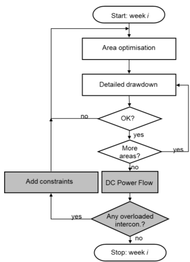
Once the Area Optimization and the Detailed Drawdown have agreed on a satisfactory solution, the functionality for detailed grid analyses in Samnett is called upon. The market solution from the Area Optimization and the Detailed Drawdown is distributed to a detailed grid model and a DC power flow solution is computed per time step within the week. Samnett checks the power flow on a user defined set of critical interconnections and registers overloads. For all interconnections being overloaded in a specific time step, power flow constraints are generated and sent back to the Area Optimization LP problem. These power flow constraints are often referred to as PTDF-constraints, where the acronym PTDF stands for power transfer distribution factors. In case of overloads, the Area Optimization and Detailed Drawdown are re-visited, as illustrated in Figure 1. This outer iteration loop is referred to as a Samnett iteration. As will be described later, it is possible to shortcut this iteration loop by adding all power flow constraints at once, i.e., not only for overloaded interconnections. However, this will increase computation time substantially.
Optionally, the user may decide to compute power losses while running the DC power flow analyses. If so, power losses per area are computed and sent to the Area Optimization. The power losses enter the Area Optimization as parameters being subtracted from the load. The possibility to compute losses internally is different from the EMPS model, where losses are typically modelled exogenously. It is important to be aware of this difference to avoid double counting the losses.
Power flow constraints in Samnett
The power flow constraints are added to the Area Optimization problem, which is formulated as an LP problem for the specific week and weather year being simulated. The constraint is formulated as:
Where the symbols have the following explanation:
Symbol |
Explanation |
Unit |
Type |
|---|---|---|---|
\(F_c^{\max-}, F_c^{\max+}\) |
Maximum allowed flow on interconnection \(c\), in the negative (\(-\)) and positive (\(+\)) direction |
MW |
Parameter |
\(f_c^0\) |
Base-case flow on interconnection \(c\) obtained from a DC power flow of the detailed transmission grid |
MW |
Parameter |
\(\phi_{ca}\) |
Zonal PTDF from area \(a\) on interconnection \(c\) |
- |
Parameter |
\(p_a^{np}\) |
Net position for area \(a\) |
MW |
Decision variable |
\(p_a^{np,0}\) |
Base-case net position for area \(a\) |
MW |
Parameter |
\(A\) |
Set of areas represented in the detailed grid |
- |
Parameter |
The maximum flow boundaries are provided by the user (file KOMBSNITT.DATA).
The base-case net positions are obtained from the last solved Area Optimization problem. The base-case flows are found after mapping the decisions from the last solved Area Optimization and the consequent Detailed Drawdown problem to the transmission grid and solving a DC power flow.
The zonal PTDFs are computed internally in Samnett based on the transmission grid data, the PTDF weighting scheme, and possible line outages.
Importantly, the net positions are the only decision variables in equation (1). Thus, one seeks to regulate the interconnection flow by adjusting the net positions in all areas that are part of the synchronous grid (1).
Although not shown in equation (1) for simplicity, slack variables are included to ensure that a feasible solution is always found. Currently, the marginal cost of using slack variables is set to a high number so that these are only used as a last resort. The user is warned when these slack variables are used.
Further information on the formulation of PTDF-constraints, loss computation, and the simulation logic in Samnett is presented in the technical report TR A7164 “Samnett – The EMPS Model with Power Flow Constraints”.
Using Samnett
Running a simulation
Include the folder with the downloaded programs in your path and go to the dataset folder. Samnett may be run by use of the program sam.exe. For running Samnett, type: sam nett on the command line.
Samnett should be seen as an additional functionality to the EMPS model. By simply running sam one will run the area simulation and Detailed Drawdown in the EMPS, similar to the program samtap.
The current version of Samnett will not work properly with all EMPS-functionality. Below is a list of known functionalities that will not work properly with Samnett:
Quadratic losses on line flows (Samnett allows one line segment only)
EIC-method (reduced availability on market options)
Controlling the input data - Wlog.txt
Samnett requires a substantial amount of additional data compared to the EMPS model. It is important that this is precise to ease the interpretation of results and to ensure that the model finds feasible solutions. Whenever changes have been made to a dataset, we recommend studying the ‘warning log’ written to the file WLog.txt when starting up the program. If one does not want to run a full simulation it is possible to write the WLog file and then exit by using the following command:
Sam NETT WLOG
Areas with and without detailed grid
A Samnett dataset is typically based on an EMPS dataset. The definition of price areas and the order in which they are enumerated is specified by the user. The recommendation in Samnett is to sort areas with detailed grid first, followed by the areas without grid. For a model of Northern Europe where the synchronous Nordic transmission grid is included, we recommend sorting the Nordic areas first.
In case this order has not been followed, it is possible to inform Samnett about the “mismatch” so that simulation is still possible. This is done by specifying the following environmental variable:
LTM_SAMNETT_EXTMODRED=TRUE
In addition, a file named ExtModred.dat should be included in the data catalogue. It comprises one line, where all areas with detailed grid description should be listed by their number in increasing order. An example line is provided below: 1,2,3,4,5,6,7,8,9,10,11,19
In this example, areas 1-11 and 19 should all be part of the detailed grid description.
If ExtModred is used, the files EFI-PREF.dat and EFI-FAST.dat should be carefully prepared so that non-grid areas are listed in between grid-areas. For the example above, areas 12-18 need to be listed in EFI-PREF and EFI-FAST although they do not have detailed grid.
File description - Wlog.txt
The simulation warning log reports errors discovered in the initial process of allocating busbars from the network model to market areas and mapping production, load, HVDC-connections and the market options to the network model. Simulation errors or peculiar simulation results can often be explained or detected by evaluating this file. The users should work with this log to keep the number of warnings as low as possible.
We have tried to classify warnings;
type 1 warnings are serious warnings/errors
type 2 warnings are less serious. Some examples are listed below:
 1 EFI-PROD-1.DAT : Busbar 55061 is assigned area  3, according to SNITT: 4
Explanation: A busbar defined electrically in area 4 (according to EFI-SNITT) receives power from a hydropower module allocated in area 3. Such inconsistencies generate a mismatch between the power balances at market and network level, which in turn may affect the convergence properties and simulation speed experienced in Samnett (the same holds true for Samlast).

 2 EFI-PROD-2.DAT : Busbar 30114 already listed
Explanation: EFI-PROD-2 couples a single hydropower module to two or more busbars by assigning a fixed share of the module’s production to each busbar. In this case, the busbar 30114 is listed several times. This is not incorrect, but does not make sense, and may indicate a modeling error.

 2 EFI-PREF.dat   : Busbar 51132 allready listed
Explanation: EFI-PREF couples a single step on the market description to one or more busbars by assigning a fixed share of the steps’s production to each busbar. In this case, the busbar 51132 is listed several times. This is not incorrect, but does not make sense, and may indicate a modeling error.

 2 EFI-PREF.dat   : Busbar 37144 in area 11 reported weight 0.0
Explanation: The busbar 37144 is assigned zero weight in EFI-PREF. This is not incorrect, but does not make sense, and may indicate a modeling error.


2 EFI-PREF.dat   : Trinn BIO_COND in area 12 is not recognized
Explanation:  EFI-PREF lists a step named “BIO_COND”, which is not found in the pre-established definition of the market description in area 12. All steps used in EFI-PREF should be found in the corresponding *.ENMD files. This step will not distribute power to its connected busbars in the simulation, as it is not found in the market model.

2 EFI-PREF.dat   : Trinn EXCH FIN-SWE in area 13 is not recognized
  -> Possible ERROR: check EXCH FIN-SWE
Explanation:  In principle the same error as above, but in this case a HVDC-connection is involved (assuming the users name these steps “EXCH” + description). The power transported to/from Finland in the market model is not received/sent in Finland in the transmission network model.

 1 KOMBSNITT.DAT  : Line 57052-30244 between areas 0 0 was not found
Explanation:  A line is listed as a part of a monitored interconnection in KOMBSNITT, but is not found in the network description.

 2 EFI-PROD-2.DAT : Busbar 37275 is not defined in network description
Explanation:  Hydropower is distributed to a busbar which is not defined in the network description.

 1 EFI-MODRED.DATA: HVDC connection     14    17
   No match in pref with EXCH DKO-FYN
   -> This step has NBus=0 and is not considered!
Explanation:  The step “EXCH DKO-FYN” defined in EFI-MODRED is not found in the pre-established market description (check corresponding *.ENMD file). The consequence is that the transported power in the market model is not distributed to the network model.

  1 EFI-SNITT connection nr. 16 has  6 lines
    identical snitt not found in KOMBSNITT
Explanation:  Mismatch between definitions of an interconnection in EFI-SNITT and KOMBSNITT.

  2 NORGESYD             - NORGEVEST
    Maske capacity =  1000.0 KOMBSNITT capacity =  2000.0
Explanation:  Mismatch between capacities defined in MASKENETT and KOMBSNITT. These should be equal.
Planned outages
Planned outages (or ‘revisions’) of transmission lines and interconnectors can be specified in many ways:
Through MASKENETT.DATA, as in the EMPS model. Such revisions will only impact the trade capacities and are not relevant if the option Relax Maske Bounds in styredata.nett is set to 2.
Through KOMBSNITT.DAT. These revisions impact the transfer limits of the interconnections as seen when checking overloads in the power flow computations. These revisions will not impact the impedances in the transmission grid and will therefore not impact computations of the PTDF matrix.
Through the file linjerevisjon.csv. These revisions will impact the grid impedance and thus also the computations of the PTDF matrix.
Using KOMBSNITT.DAT
The file format of KOMBSNITT.DAT is explained in KOMBSNITT.DAT. It provides a set of interconnections that are monitored for overloads. The N first interconnections should be identical to the interconnections provided in EFI-SNITT.DAT. These define the electrical division of areas. We refer to these as pure interconnections, always comprising lines that connect two areas.
Following the N pure interconnections in KOMBSNITT, a set of combined interconnections can be added. These are optional and there are no strict rules regarding the lines that are included in a combined interconnection. Some possible uses of combined interconnections are discussed below.
Interconnections with Internal Lines
Some interconnections may fully or partially consist of lines that are internal in an area. These represent corridors that are important to monitor when operating the grid. It is important that such interconnections are electrically close to area borders to ensure that controlling their flow by PTDF-constraints is possible at reasonable cost.
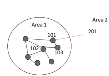
An illustrative example is provided in the following, where the sum of flows on two lines is monitored. The interconnection is named SNITT A and comprises lines spanning busbars 101-201 and 102-103 as defined below:
'SNITT A',' ',
2,1000,1000,0,
101,201,1,1,
102,103,1,1,
The lines in interconnection SNITT A are shown as dotted red lines in Figure 2. The electrical area definition for Area 1 is illustrated by the black circle. While line 101-201 connects Area 1 with Area 2, line 102-103 connects busbars internally in Area 1. This type of interconnection may be important to include to properly constrain the market solution, but the control of flow on internal lines, such as 102-103 in this example, may be challenging though use of PTDFs per area. It could be that the PTDF of Area 1 on the flow from Area 1 - Area 2 is positive while the PTDF of Area 1 on the flow from 102 - 103 is negative. If that is the case, controlling the flow on SNITT A will be expensive and possible infeasible. The user could obtain information about challenging interconnections through the files PTDF.csv, NettDual.dat, NettDual.csv, and FlytAvvikdat.
|
|---|
Security constraints
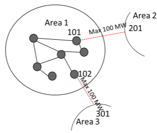
One can formulate interconnections that implicitly consider the possibility of line outages. An illustrative example is provided in the following, where the sum of flows on two lines is monitored. The interconnection is named SNITT B and comprises lines spanning busbars 101-201 and 102-301 as defined below:
'SNITT B',' ',
2,100,100,0,
101,201,1,1,
102,301,1,1,
Although the maximum flow capacity on each line is 100 MW, the definition of SNITT B only allows 100 MW on the sum of the two. This interconnection will then secure a market solution that allows one of the two lines to be out of operation.
|
|---|
Using EFI-AREA for aggregation to price areas
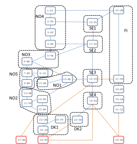
The file EFI-AREA.DAT allows the user to group modelled areas to form larger (or aggregated) price areas. This is illustrated in Figure 4, where for example a new aggregated price area NO4 is created by grouping the modelled areas 1-4. If EFI-AREA.DAT is used, Samnett will compute zonal PTDFs for the aggregated price zones.
|
|---|
The feature allows model users to resemble the price formation in a market based on flow-based market clearing and zonal pricing. There are, however, some potential challenges by using this functionality:
The precision in the regulation of overloads generally decreases with increasing size of the price zones. Additionally, more of the monitored interconnections are likely to be located within a zone, which further complicates the control of power flow through PTDF-constraints.
The “marginal cost” of hydropower (water values) are computed per modeled area. Differences in water values within an aggregated price zone may lead to results that are difficult to interpret.
Output to screen
Samnett will print information to screen while running. Below is a short description of some of the information that is presented.
First, the program name and version are printed. Knowing the program version is important when reporting possible bugs to SINTEF.
S A M N E T T _ H P O - -verno- - -dato-
After reading the EMPS input data, Samnett starts reading the grid data and coupling files and echoes this process to screen:
 Reading: MyGrid.sav
 Retrieving PSSE-data:  10177 buses
                       12189 branches
 Completed reading PSSE-data
 SwingBus:        55059

 Reading: EFI-SNITT.DAT
 Coupling busbars to areas
 Reading: EFI-PROD-1.DAT
 Reading: EFI-PROD-2.DAT
 Reading: EFI-PREF.DAT
 Reading: EFI-FAST.DAT
 Reading: EFI-VIND.DAT
 Coupling preference and firm-power steps to areas
 Reading: KOMBSNITT.DAT
 Reading: MODRED.DATA
 Reading: EFI-AREA.DAT
   ... not present
 Reading: LINJEREVISJON.CSV
   ... not present
 Completed reading of network data
The runtime environment defined by LTM passwords are stored in the file RunInfo.txt. This information is useful for debugging purposes.
Subsequently, the control parameters provided in the file styredata.nett are echoed to screen.
 TAPSBEREGN      =   T
                >=   200 kV
 NORDELTAP       =   T
 MARGLOSS        =   F
 PHASESHIFT      =   F
 FBMCPARAM       =   T
 Successive LP   =   F
 No relaxation   =   F
 MaxOverload     =   2.0 %
 RelaxBounds     =   0
 PTDF-weight     =   0
 MaxIterNett     =   15

EFI-VIND coupled    6 out of 191 wind series to nodes
The last line shows the number of wind series that are successfully coupled to busbars in the transmission grid through EFI-VIND.dat.
Reading file : griddata_dump.nett
for dumping of grid results to GRIDDUMP.h5
The two lines above indicates that detailed grid results are written to file according to the specification in griddata_dump.nett, se Section TODO for more information on the formats.
Next, Samnett reports from the simulation, stating the inflow year being simulated (here: 1988), followed by the week number (1), the number of iterations between the EMPS model (Area Optimization/Detailed Drawdown) and the DC power flow analysis (4), and finally the sum of iterations internally in the EMPS model between the Area Optimization and the Detailed Drawdown model (207). The number of iterations between the EMPS model and the DC power flow is worth keeping an eye on since it provides a measure for the tightness of the grid constraints in KOMBSNITT.DAT.
Simulering av scenario nr:  1 1988
uke =     1    4  207
Sometimes a star (*) is written for one or several weeks, e.g.:
uke = 31 15 807 *
This means that the Area Optimization problem including the PTDF-constraints is not feasible, and that slack variables have been used related to one or more PTDF-constraint to ensure feasibility. The use of these slack variables has a very high cost which in turn will be reflected in the simulated power prices. The user should therefore be careful when interpreting the results from a simulation if use of such slack variables has been reported.
Bibliography
[1] Helseth, A., “User’s guide to Samnett” 2025.